Understanding Present Value Interest Factor (PVIF) is essential in financial analysis, as it helps determine the current worth of future cash flows. Fortunately, Excel makes calculating PVIF a breeze, allowing you to analyze investments, loans, and other financial situations easily.
What is PVIF?
In finance, the Present Value Interest Factor (PVIF) is crucial in evaluating investments, analyzing loans, and making informed financial decisions. It allows us to bridge the gap between future cash flows and their current worth, accounting for the ever-important time value of money.
Understanding the Time Value of Money
Imagine receiving $100 today compared to receiving $100 a year from now. While the amount seems identical, the value differs significantly. Money’s time value dictates that a dollar received today is worth more than a dollar received in the future, primarily due to the potential for earning interest or returns.
Introducing PVIF: Bridging the Gap
PVIF serves as a discount factor that allows us to translate future cash flows to their equivalent present value. It essentially “discounts” the future value back to today’s worth, considering the prevailing interest rate and the number of periods until the cash flow is received.
The PVIF Formula
The PVIF formula is:
PVIF = 1 / (1 + r)^n
Where:
- r is the discount rate per period
- n is the number of periods
Example
For instance, if you want to calculate the PVIF for a cash flow that will occur 5 years from now with a discount rate of 6%, the formula would be:
PVIF = 1 / (1 + 0.06)^5
How to Calculate PVIF in Excel?

1. Setting Up Your Excel Sheet
Step 1: Open a new Excel workbook.
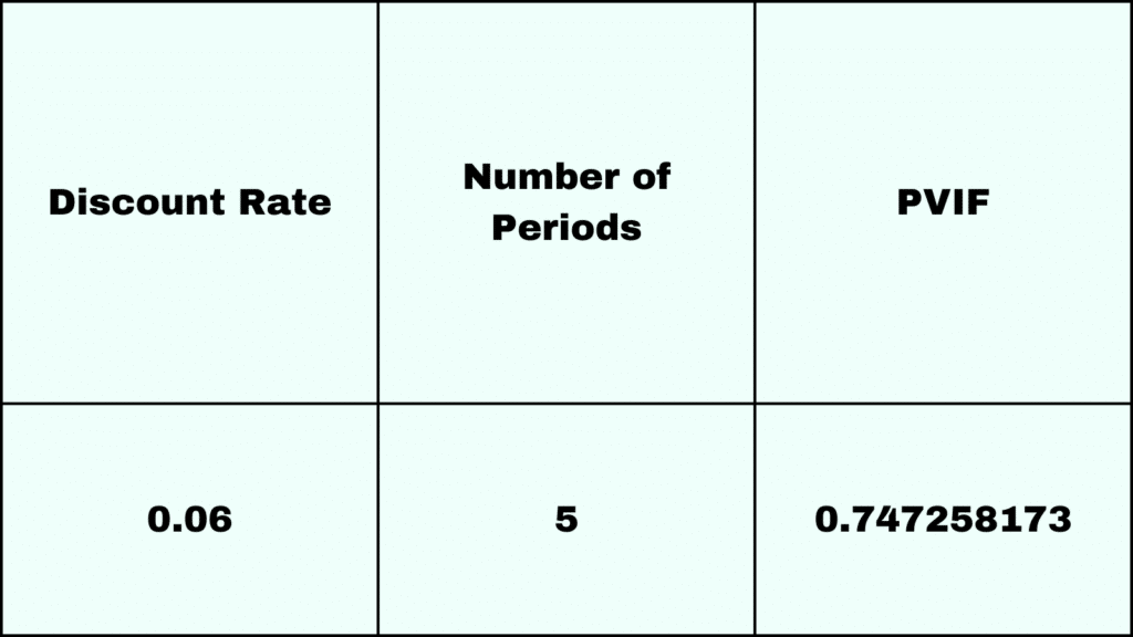
Step 2: In cell A1, type Discount Rate.
Step 3: In cell B1, type Number of Periods.
Step 4: In cell C1, type PVIF.
2. Entering Data and Formulas
Step 5: Enter the discount rate in cell A2. For example, input 0.06 for a 6% rate.
Step 6: In cell B2, input the number of periods, such as 5 for 5 years.
Step 7: In cell C2, enter the formula =1/(1+A2)^B2.
3. Calculating the PVIF
Step 8: After entering the formula in cell C2, press Enter. Excel will compute the PVIF.
4. Example Result and Interpretation
Excel will display a value in cell C2. For this example, the result is approximately 0.7473.
This PVIF value of 0.7473 means that one dollar received 5 years from now is worth approximately 74.73 cents in today’s terms, considering a 6% annual discount rate.
5. Adjusting and Reusing the Formula
Step 9: You can adjust the numbers in cells A2 and B2 for different scenarios, and the formula in C2 will automatically update the PVIF. This flexibility allows for easy analysis of various financial situations.


