To calculate the Future Value Interest Factor of Annuity (FVIFA) in Excel, we must first grasp the Future Value Interest Factor (FVIF) formula.
The formula is:
FVIFA = [(1 + r)^n – 1] / r
Where:
- “r” is the interest rate per period.
- “n” is the number of periods.
In Excel, you can easily compute FVIFA by following the steps below.

Step 1. Input Data
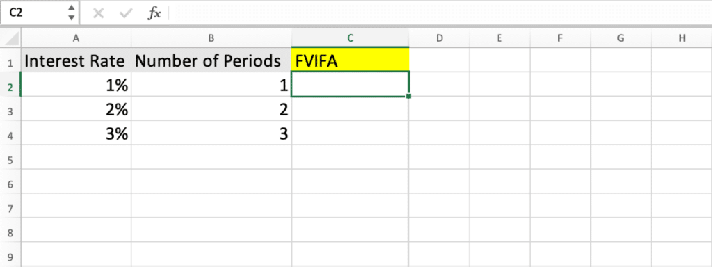
To calculate FVIFA in Excel, you need to set up your spreadsheet with the necessary data.
In the spreadsheet, select two separate cells to enter the fundamental inputs: the annual interest rate and the number of periods. For example, in cell A1, type “Interest Rate,” and in cell B1, type “Number of Periods.” Below each header, input your data. (This structure is very simple. If you need a table of FVIFA for various combinations, you can directly skip to Step 3.)
Step 2. Formula Application
Once you’ve set up your data with headers and inputs, the next step is to use the FVIFA formula in Excel.
Select a new cell where you want the FVIFA result to appear. Let’s say it is cell C2, right next to your input data.
In the chosen cell, enter the FVIFA formula we introduced in the opening paragraph of this article. For instance, if your interest rate is in cell A2 and the number of periods is in cell B2, your formula in cell C2 would be “=((1+A2)^B2-1)/A2”.
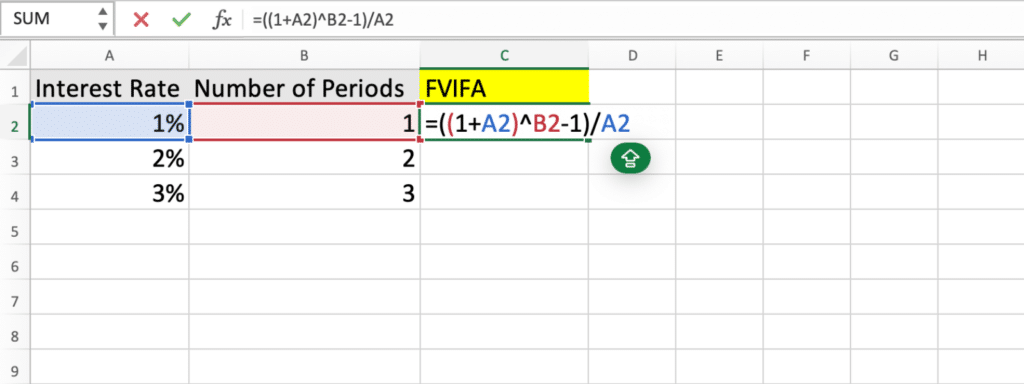
Press Enter after typing the formula. Excel will calculate the FVIFA based on your inputs. Drag down and the FVIFA for the interest rates and numbers of periods in cells below will automatically show up.
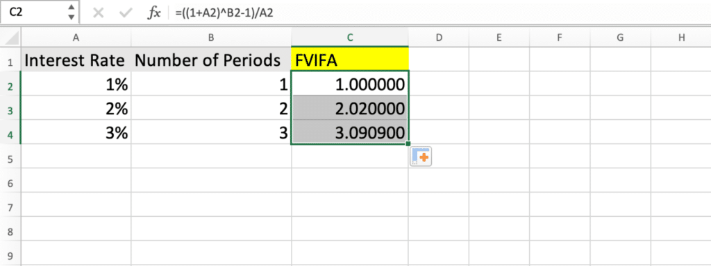
You can now change the values in column A and column B to see how different interest rates and periods affect the FVIFA. Easy, huh?
Step 3. Make a FVIFA Table (Optional)
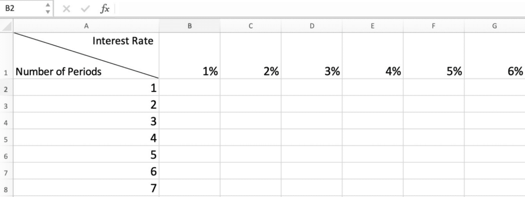
Creating an FVIFA table in Excel with periods in column A and interest rates in row 1 requires a slight modification of our method. Here’s how to do it:
- Set Up the Table: In column A, starting from cell A2, list the number of periods (1, 2, 3, etc.). In row 1, starting from cell B1, list the interest rates (like 1%, 2%, 3%, etc.).
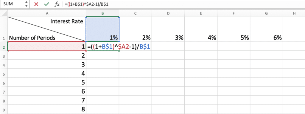
Creating FVIFA Table in Excel – Step 3 – 1 - Enter the FVIFA Formula: Select the cell B2 (the intersection of your first interest rate and the first period). Enter the formula “=((1+B$1)^$A2-1)/B$1”. Here, B$1 references the interest rate in the first row and remains constant horizontally. $A2 references the number of periods in the first column and remains constant vertically.
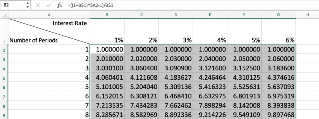
Creating FVIFA Table in Excel – Step 3 – 2 - Use the Formula Across the Table: Drag the fill handle (the small square at the bottom-right corner of cell B2) across the row to fill the formula for other interest rates. Then, drag the fill handle down the column to apply the formula for other periods.
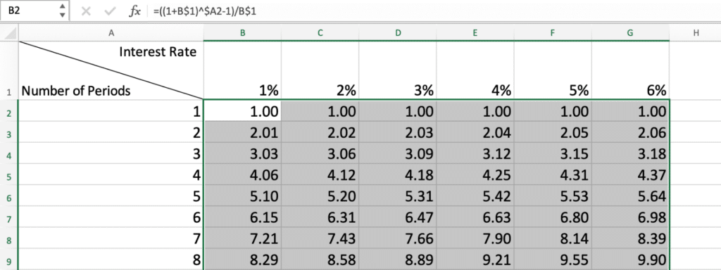
Creating FVIFA Table in Excel – Step 3 – 3 - Format the Table: Format the interest rate cells to display percentages and the FVIFA cells to show the desired number of decimal places.
Creating FVIFA Table in Excel – Step 3 – 4
Now, your table shows the FVIFA for different combinations of interest rates and periods. Change values in the interest rate row or the number of periods column to see how FVIFA adjusts!


