The 7-Day Yield is crucial for evaluating short-term investment returns, particularly in money market funds. This article provides a straightforward guide on how to calculate the 7-Day Yield using Excel, a common tool for financial analysis.
The 7-Day Yield Formula
The formula to calculate the 7-Day Yield is a key tool for investors to understand the potential annualized return for a money market mutual fund based on a week’s performance. It is expressed as:
7-Day Yield (%) = ((End Price + Distributions – Start Price – Fees) / Start Price) * (365/7)
- End Price + Distributions: This represents the value of a share, including earnings (such as dividends or interest), at the end of the seven days.
- Start Price: The value of the share at the beginning of the seven days.
- Fees: These are the fees incurred during the seven-day period, which may include management fees or other charges.
- Annualizing Factor (365/7): This converts the weekly yield into an annualized figure, providing a hypothetical yearly rate if the week’s performance were to continue unchanged for an entire year.
Calculating the 7-Day Yield in Excel: A Detailed Example

Assume you want to calculate the 7-Day Yield for two money market mutual funds using Excel. Here’s how to set it up and get your results:
Setting Up the Worksheet:
Adjust the width of columns A, B, and C for better visibility.
Label column B as ‘Fund A’ and column C as ‘Fund B’.
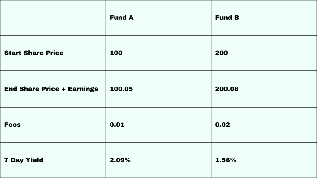
For example, let’s consider two hypothetical money market funds: Fund A and Fund B. Fund A has an end share price (including earnings) of $100.05, a start share price of $100, and incurs $0.01 in fees. Fund B has an end share price of $200.08, a start share price of $200, and incurs $0.02 in fees.
Entering Data:
In cells A2, A3, and A4, enter ‘Start Share Price’, ‘End Share Price + Earnings’, and ‘Fees’, respectively.
Enter ‘7-Day Yield’ in cell A5.
Inputting the Numbers for Fund A:
In cell B2 (Start Share Price), enter 100.
In cell B3 (End Share Price + Earnings), enter 100.05.
In cell B4 (Fees), enter 0.01.
Calculating the 7-Day Yield for Fund A:
In cell B5, input the formula =((B3 – B2 – B4) / B2) * 365/7.
This formula will calculate the 7-Day Yield for Fund A.
Repeating the Process for Fund B:
Input 200 in cell C2, 200.08 in cell C3, and 0.02 in cell C4.
In cell C5, use the formula =((C3 – C2 – C4) / C2) * 365/7 to calculate the 7-Day Yield for Fund B.
Interpreting Results:
The values in cells B5 and C5 give each fund’s annualized 7-Day Yield, reflecting the projected yearly return based on the past week’s performance.
For Fund A, the 7-Day Yield is approximately 2.09%.
For Fund B, the 7-Day Yield is also approximately 1.56%.
This Excel method offers a precise and efficient way to calculate and compare the 7-Day Yield of different money market mutual funds, aiding in financial analysis and decision-making.
Related Calculator:


